Baseline model reproduction

The fixed clinical equation and its fitted predictor correlation

ImportantThe copula is now a sensitivity analysis

The real joint distribution of the predictors became available after the lock, and the copula turned out to be 10% of probability mass away from it. Since decisions D8, D9 and D10 (18 October 2026) the baseline cohort is the observed distribution of the 128 profiles in the 4,078 unique admissions of boscore.xlsx, the baseline model is a refit on it (next section), and everything else on this page describes the published equation and the copula that are kept as sensitivity analyses. See the comparison with the real data.

source("_setup.R")
rep  <- read.csv("output/reproduction_report.csv")
loss <- read.csv("output/reproduction_loss.csv")
cmp  <- read.csv("output/fit_comparison.csv")

The refit baseline (D10)

The baseline model is a maximum-likelihood logistic refit of the seven predictors on the 4,078 unique admissions in 1,945 patients. It is fixed from here on, and genetic terms will be fitted on top of it. Standard errors are clustered by patient, and the bootstrap resamples patients and repeats the refit in every resample.

rp <- read.csv("output/baseline_refit_parameters.csv")
rp |>
  transmute(Term = gsub("_", " ", term), Published = published, Refit = refit, `Robust SE` = se_robust,
            `Bootstrap 5%` = lo, `Bootstrap 95%` = hi, `Odds ratio` = ifelse(term == "(Intercept)", NA, odds_ratio)) |>
  gt() |>
  fmt_number(2:6, decimals = 2) |>
  fmt_number(7, decimals = 2) |>
  sub_missing(missing_text = "")

Table 1: Refit coefficients against the published ones. Every published coefficient lies inside the refit’s 90% bootstrap interval.

Term	Published	Refit	Robust SE	Bootstrap 5%	Bootstrap 95%	Odds ratio
(Intercept)	−5.45	−5.59	0.27	−6.13	−5.22
uncontrolled malignancy	0.68	0.76	0.20	0.44	1.11	2.15
high risk chemo	0.79	0.86	0.24	0.49	1.26	2.37
high dose steroids	0.80	0.80	0.25	0.34	1.20	2.23
severe lymphopenia	0.89	0.93	0.23	0.56	1.32	2.54
cmv	1.14	1.42	0.32	0.85	1.96	4.14
prolonged neutropenia	1.52	1.58	0.29	1.13	2.10	4.83
prior mould disease	1.64	1.99	0.28	1.50	2.47	7.28

read.csv("output/baseline_refit_performance.csv") |>
  transmute(Metric = metric, Apparent = apparent, Optimism = optimism, Corrected = corrected) |>
  gt() |>
  fmt_number(2:4, decimals = 4)

Table 2: Performance of the refit baseline. Optimism is reported and not subtracted.

Metric	Apparent	Optimism	Corrected
aROC	0.8577	0.0046	0.8531
calibration slope	1.0000	0.0288	0.9712
mean predicted risk	0.0326	0.0000	0.0326
observed prevalence	0.0326	0.0000	0.0326
observed net benefit at 5%	0.0152	0.0005	0.0148
observed net benefit at 10%	0.0086	0.0007	0.0079
observed net benefit at 20%	0.0040	0.0007	0.0033

The refit is calibrated in the large by construction, and the optimism is small: aROC falls from 0.858 to 0.853 and the calibration slope is 0.97. The published equation is kept as a sensitivity analysis, described in the rest of this page.

The published equation (sensitivity analysis)

This is the Stanzani et al. (2019) equation. Until decision D10 it was the fixed clinical block.

\[ \operatorname{logit}(p) = -5.45 + 0.68\,\text{malignancy} + 0.79\,\text{chemo} + 0.80\,\text{steroids} + 0.89\,\text{lymphopenia} + 1.14\,\text{CMV} + 1.52\,\text{neutropenia} + 1.64\,\text{prior mould} \]

Exponentiating each coefficient reproduces the published adjusted odds ratios in Table 2.

data.frame(
  Predictor = gsub("_", " ", PREDICTORS),
  Coefficient = pars$coef[PREDICTORS],
  `Odds ratio` = exp(pars$coef[PREDICTORS]),
  `In cases` = pars$prev_case[PREDICTORS],
  `In non-cases` = pars$prev_non[PREDICTORS],
  Overall = pars$marginal[PREDICTORS],
  check.names = FALSE
) |>
  gt() |>
  fmt_number(2:3, decimals = 2) |>
  fmt_percent(4:6, decimals = 1)

Table 3: Published predictors. Prevalences are in IMD cases (n = 133), non-cases (n = 3,994) and overall (n = 4,127 admissions).

Predictor	Coefficient	Odds ratio	In cases	In non-cases	Overall
uncontrolled malignancy	0.68	1.97	58.7%	40.6%	41.2%
high risk chemo	0.79	2.20	63.9%	19.4%	20.9%
high dose steroids	0.80	2.23	22.6%	10.9%	11.3%
severe lymphopenia	0.89	2.44	48.9%	11.6%	12.8%
cmv	1.14	3.13	12.8%	2.4%	2.7%
prolonged neutropenia	1.52	4.57	79.7%	27.5%	29.2%
prior mould disease	1.64	5.16	15.0%	2.2%	2.6%

What has to be reproduced

A synthetic cohort must reproduce 16 published targets: the IMD prevalence, the aROC, and the prevalence of each predictor separately in cases and non-cases. The paper does not publish the joint distribution of the seven predictors, and it is load-bearing. High-risk chemotherapy and prolonged neutropenia, for example, are close to the same clinical state and cannot be drawn independently.

I model the joint with a Gaussian copula: each predictor is a thresholded latent normal variable that keeps its published marginal prevalence, and the correlation of the latent variables is the assumption to be calibrated. Because the predictors are binary, every quantity of interest is a function of the 128 predictor profiles. The profile probabilities are computed by numerical integration of the 7-dimensional normal, so no patient-level sampling enters the results below.

Reproduction

g <- rep[rep$target %in% c("prevalence", "aroc"), ]
ch <- setNames(loss$chi2, loss$model)
pct <- function(x) sprintf("%.2f%%", 100 * x)
tibble(
  Quantity = c("IMD prevalence", "aROC", "Chi-square, 16 targets"),
  Published = c(sprintf("%.1f%%", 100 * g$published[1]), sprintf("%.3f", g$published[2]), "0"),
  Independence = c(pct(g$independent[1]), sprintf("%.3f", g$independent[2]), sprintf("%.0f", ch[["independent"]])),
  `Exchangeable rho = 0.30` = c(pct(g$exchangeable_0.30[1]), sprintf("%.3f", g$exchangeable_0.30[2]),
                                sprintf("%.0f", ch[["exchangeable_0.30"]])),
  `Fitted v1` = c(pct(g$fitted_v1[1]), sprintf("%.3f", g$fitted_v1[2]), sprintf("%.1f", ch[["fitted_v1"]])),
  `Fitted v2` = c(pct(g$fitted[1]), sprintf("%.3f", g$fitted[2]), sprintf("%.2f", ch[["fitted"]]))
) |> gt()

Table 4: Global targets under five joint distributions. Chi-square sums squared errors, in published standard errors, over all 16 targets.

Quantity	Published	Independence	Exchangeable rho = 0.30	Fitted v1	Fitted v2
IMD prevalence	3.3%	2.24%	3.27%	3.25%	3.22%
aROC	0.850	0.775	0.854	0.848	0.849
Chi-square, 16 targets	0	346	47	8.6	0.36

NoteThe 3.3% prevalence target

133 of 4,127 admissions is 3.22%, not 3.3%. The 3.3% figure was kept as pre-specified (decision D6). The difference is about 0.3 standard errors and does not affect the fit.

Independence gives the right per-predictor prevalences by construction but a prevalence of 2.2% and an aROC of 0.775. A single exchangeable correlation of 0.30 recovers both global targets but misses several case-group prevalences. The structured fits do better on both counts.

lab <- gsub("_", " ", sub("^noncase_prev:", "non-case: ", sub("^case_prev:", "case: ", rep$target)))
rep |>
  transmute(target = factor(lab, levels = rev(lab)),
            `Exchangeable rho = 0.30` = z_exchangeable, `Fitted v1` = z_fitted_v1, `Fitted v2` = z_fitted) |>
  pivot_longer(-target, names_to = "model", values_to = "z") |>
  mutate(model = factor(model, c("Exchangeable rho = 0.30", "Fitted v1", "Fitted v2"))) |>
  ggplot(aes(z, target, colour = model)) +
  geom_vline(xintercept = c(-2, 2), linetype = "dashed", colour = jama_cols[["grey"]]) +
  geom_point(size = 2.2) +
  scale_colour_manual(values = c("Exchangeable rho = 0.30" = jama_cols[["grey"]], "Fitted v1" = jama_cols[["steel"]], "Fitted v2" = jama_cols[["navy"]])) +
  labs(x = "Standard errors from the published value", y = NULL, colour = NULL) +
  theme_jama(grid = "x")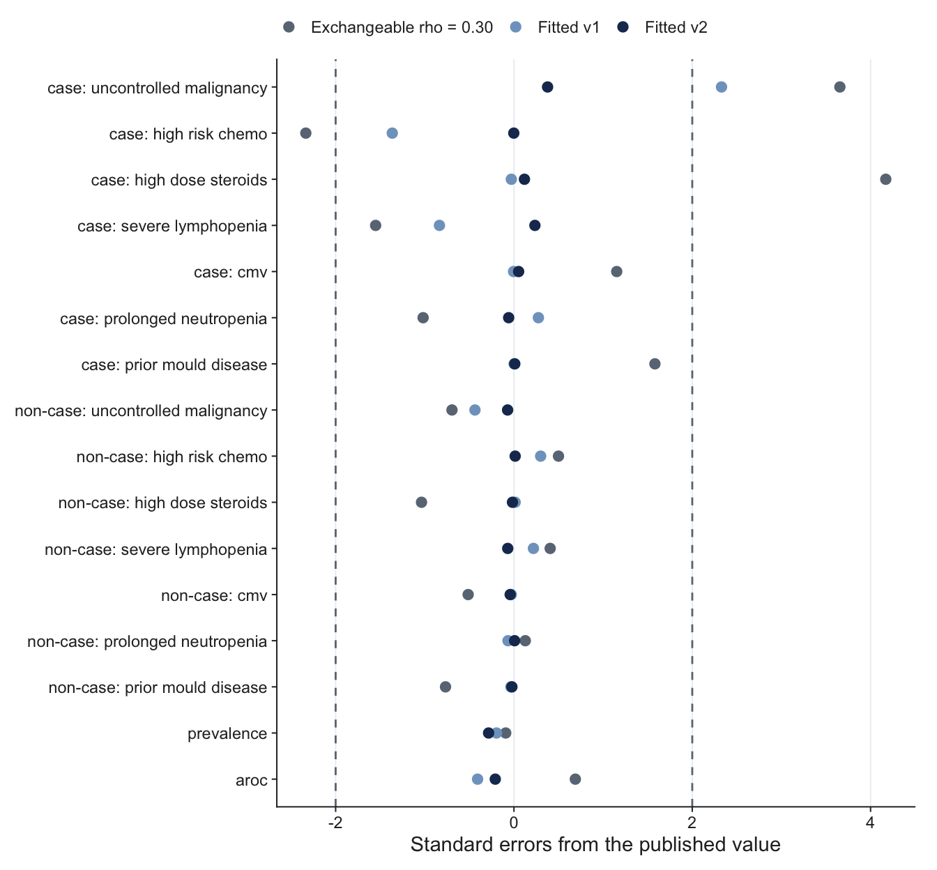

Figure 1: Simulated minus published value, in published standard errors, for each of the 16 targets. Dashed lines mark two standard errors. Independence is omitted because it is far outside this range.

The fitted correlation structure

The matrix is structured by clinical grouping, with non-negative dependence. The marrow-suppression block (malignancy, chemotherapy, lymphopenia, neutropenia) shares a baseline correlation, with extra correlation allowed for the pairs that the requested Bologna cross-tabulations would cover. Steroids, CMV and prior mould disease are tied to the block by single parameters.

Version 1 and what went wrong with it

Version 1 had eight parameters. It left uncontrolled malignancy in cases simulated at 69% against 59% published (2.3 standard errors), and two block parameters sat at their upper bound. Both problems had one cause. Neutropenia is tightly tied to both chemotherapy and lymphopenia, which forces chemotherapy and lymphopenia to be correlated for the matrix to stay positive definite. In version 1 that pair shared the block baseline with malignancy’s links, so raising the baseline to satisfy the first pulled malignancy up with it.

Version 2 gives chemotherapy-lymphopenia its own parameter and lets the three block extras reach 0.7.

cmp |>
  transmute(
    Model = recode(config,
                   v1 = "v1: 8 parameters, extras capped at 0.5",
                   v2_capped = "v2 with the v1 caps (9 parameters)",
                   v2 = "v2: 9 parameters, extras capped at 0.7"),
    `Chi-square` = chi2, Prevalence = prevalence, aROC = auc,
    `Malignancy in cases (z)` = z_malignancy_case, `Largest |z|` = max_abs_z,
    `At a bound` = gsub("; ", ", ", at_bound)
  ) |>
  gt() |>
  fmt_number(c(`Chi-square`, `Malignancy in cases (z)`, `Largest |z|`), decimals = 2) |>
  fmt_percent(Prevalence, decimals = 2) |>
  fmt_number(aROC, decimals = 3)

Table 5: Three fitted configurations, evaluated by numerical integration.

Model	Chi-square	Prevalence	aROC	Malignancy in cases (z)	Largest |z|	At a bound
v1: 8 parameters, extras capped at 0.5	8.60	3.25%	0.848	2.33	2.33	d_malig_chemo, d_chemo_neut, d_neut_lymph
v2 with the v1 caps (9 parameters)	2.74	3.21%	0.849	1.44	1.44	d_malig_chemo, d_chemo_neut, d_neut_lymph, d_chemo_lymph
v2: 9 parameters, extras capped at 0.7	0.36	3.22%	0.849	0.38	0.38	d_malig_chemo, d_chemo_neut

The malignancy residual goes away (2.3 to 0.4 standard errors). The new parameter alone, with the old caps, gets most of the way (1.4); raising the caps finishes it.

Fitted version 2

Rm <- as.matrix(read.csv("output/fitted_correlation_matrix.csv", row.names = 1))
nm <- gsub("_", " ", rownames(Rm))
long <- expand.grid(row = nm, col = nm)
long$r <- as.vector(Rm)
ggplot(long, aes(col, row, fill = r)) +
  geom_tile(colour = "white") +
  geom_text(aes(label = sprintf("%.2f", r)), size = 3) +
  scale_fill_gradient(low = "white", high = jama_cols[["steel"]], limits = c(0, 1)) +
  scale_y_discrete(limits = rev(nm)) +
  labs(x = NULL, y = NULL, fill = "Latent\ncorrelation") +
  theme_jama(grid = "none") + theme(axis.text.x = element_text(angle = 40, hjust = 1), legend.position = "right")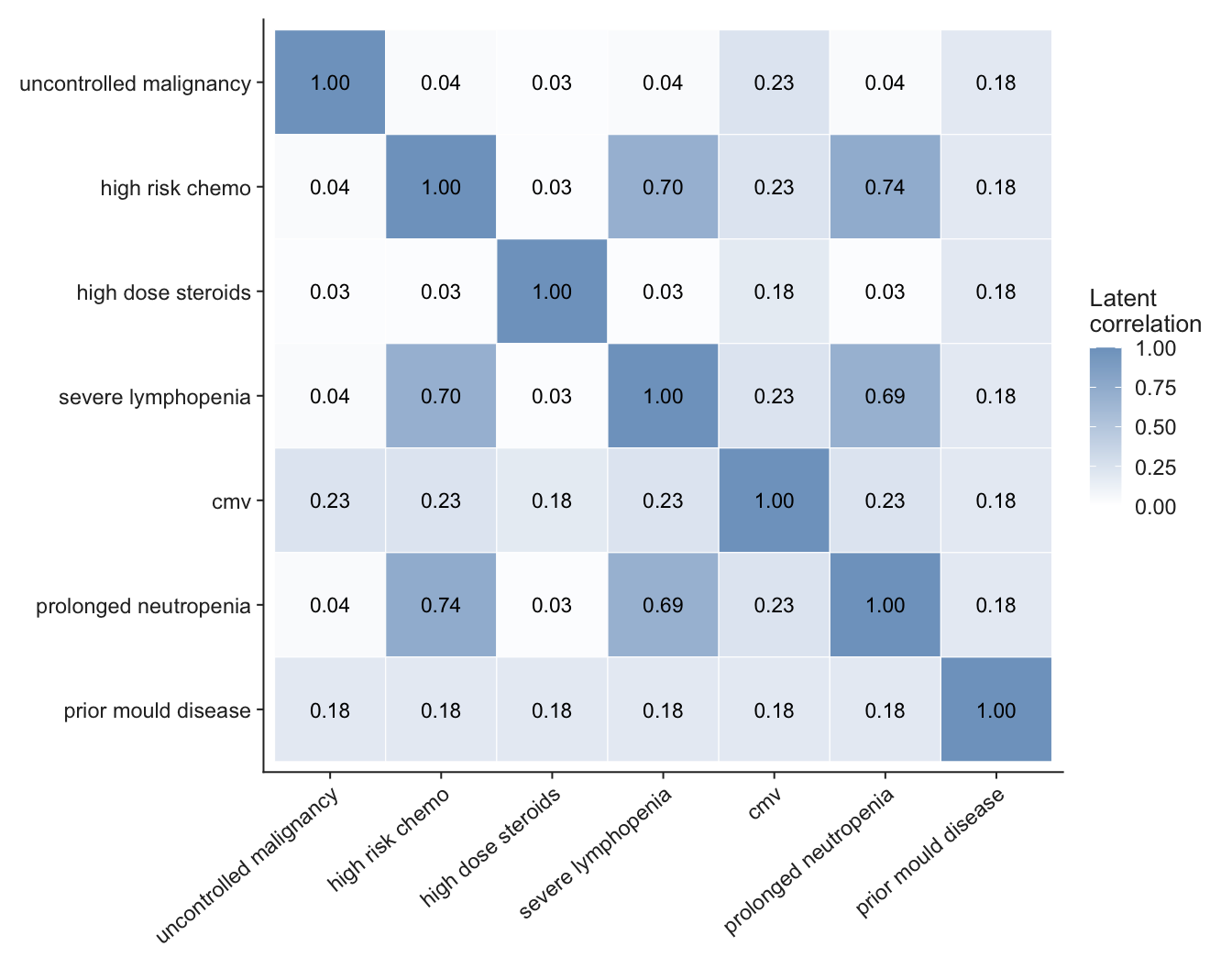

Figure 2: Fitted latent correlation matrix, version 2.

meaning <- c(
  "Baseline correlation within the marrow-suppression block (this sets malignancy's links)",
  "Extra: malignancy and chemotherapy",
  "Extra: chemotherapy and neutropenia",
  "Extra: neutropenia and lymphopenia",
  "Extra: chemotherapy and lymphopenia (new in v2)",
  "Block with high-dose steroids",
  "Block with CMV",
  "Steroids with CMV",
  "Prior mould disease with every other predictor"
)
th <- read.csv("output/fitted_theta.csv")
th$lower <- THETA_LOWER[th$parameter]
th$upper <- THETA_UPPER[th$parameter]
th$bound <- ifelse(abs(th$value - th$lower) < 0.01, "at lower bound",
                   ifelse(abs(th$value - th$upper) < 0.01, "at upper bound", ""))
th$meaning <- meaning
th |>
  select(Parameter = parameter, Meaning = meaning, Value = value, Lower = lower, Upper = upper, Note = bound) |>
  gt() |>
  fmt_number(c(Value, Lower, Upper), decimals = 2)

Table 6: Fitted parameters, version 2, and their bounds.

Parameter	Meaning	Value	Lower	Upper	Note
rho_A	Baseline correlation within the marrow-suppression block (this sets malignancy's links)	0.04	0.00	0.80
d_malig_chemo	Extra: malignancy and chemotherapy	0.00	0.00	0.50	at lower bound
d_chemo_neut	Extra: chemotherapy and neutropenia	0.70	0.00	0.70	at upper bound
d_neut_lymph	Extra: neutropenia and lymphopenia	0.66	0.00	0.70
d_chemo_lymph	Extra: chemotherapy and lymphopenia (new in v2)	0.67	0.00	0.70
rho_A_steroid	Block with high-dose steroids	0.03	0.00	0.80
rho_A_cmv	Block with CMV	0.23	0.00	0.80
rho_steroid_cmv	Steroids with CMV	0.18	0.00	0.80
rho_prior	Prior mould disease with every other predictor	0.18	0.00	0.50

Malignancy is almost uncorrelated with the other block members (latent correlation about 0.04), while chemotherapy, neutropenia and lymphopenia are correlated at 0.69 to 0.74 with each other. That is what the published figures imply under this structure. It should be checked against the requested Bologna cross-tabulation of malignancy by chemotherapy.

Is the cap on d_chemo_neut costing anything?

d_chemo_neut sits at its upper bound of 0.7. Moving it away from the fitted value, with every other parameter held, shows whether the bound is binding.

set.seed(7461)
Zs <- matrix(rnorm(3e5 * 7), 3e5)
obj <- make_objective(Zs, pars, targets)
th_fit <- setNames(th$value, th$parameter)[THETA_NAMES]
vals <- c(0.5, 0.6, 0.7, 0.8, 0.9)
tibble(`d_chemo_neut` = vals,
       `Latent chemo-neutropenia correlation` = th_fit[["rho_A"]] + vals,
       Loss = sapply(vals, \(v) obj(replace(th_fit, "d_chemo_neut", v)))) |>
  gt() |>
  fmt_number(c(`Latent chemo-neutropenia correlation`, Loss), decimals = 2)

Table 7: Fitting loss as d_chemo_neut varies, other parameters held at their fitted values (common random draws, so values differ slightly from the exact chi-square).

d_chemo_neut	Latent chemo-neutropenia correlation	Loss
0.5	0.54	3.73
0.6	0.64	1.61
0.7	0.74	0.54
0.8	0.84	0.98
0.9	0.94	3.52

The loss is lowest at 0.7 and rises on both sides, so the optimum is at the cap by coincidence and the cap is not constraining the fit. The matrix is also well inside the positive-definite region (smallest eigenvalue 0.26), so positive definiteness no longer limits the fit either.

WarningA near-zero chi-square is expected here and does not validate the structure

The 16 targets are not independent. Given the marginals, the non-case prevalences follow from the case prevalences and the overall prevalence, which leaves about nine effective constraints. Version 2 has nine parameters. A saturated fit reproduces its targets almost exactly whether or not the structure is right. Only information beyond the published margins, such as the Bologna cross-tabulations, can test it.

How well is the matrix identified?

Many matrices fit the targets about equally well. A random-walk Metropolis sampler on \(\exp(-\chi^2/2)\) gives an ensemble of near-optimal matrices (six chains, 400 retained draws each after thinning). It is not a formal posterior: the chi-square uses published sampling errors and ignores admission clustering.

raw <- read.csv("output/correlation_ensemble_raw.csv")
rhat <- function(x, chain) {
  s <- split(x, chain); n <- length(s[[1]])
  W <- mean(sapply(s, var)); B <- n * var(sapply(s, mean))
  sqrt(((n - 1) / n * W + B / n) / W)
}
summ <- tibble(
  parameter = THETA_NAMES,
  q05 = sapply(THETA_NAMES, \(p) quantile(raw[[p]], 0.05)),
  median = sapply(THETA_NAMES, \(p) median(raw[[p]])),
  q95 = sapply(THETA_NAMES, \(p) quantile(raw[[p]], 0.95)),
  rhat = sapply(THETA_NAMES, \(p) rhat(raw[[p]], raw$chain))
)
ggplot(summ, aes(median, factor(parameter, rev(THETA_NAMES)))) +
  geom_pointrange(aes(xmin = q05, xmax = q95), colour = jama_cols[["navy"]]) +
  labs(x = "Parameter value", y = NULL) +
  theme_jama(grid = "x")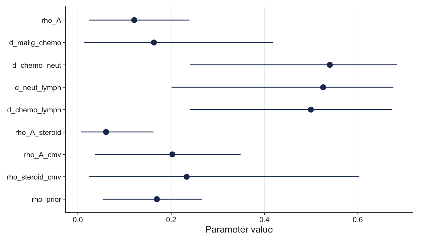

Figure 3: Median and 90% range of each parameter across the ensemble.

summ |>
  select(Parameter = parameter, `5%` = q05, Median = median, `95%` = q95, `R-hat` = rhat) |>
  gt() |>
  fmt_number(2:5, decimals = 2)

Table 8: Ensemble summaries. R-hat above about 1.1 means the chains have not fully mixed.

Parameter	5%	Median	95%	R-hat
rho_A	0.02	0.12	0.24	1.02
d_malig_chemo	0.01	0.16	0.42	1.03
d_chemo_neut	0.24	0.54	0.68	1.02
d_neut_lymph	0.20	0.53	0.68	1.04
d_chemo_lymph	0.24	0.50	0.67	1.09
rho_A_steroid	0.01	0.06	0.16	1.00
rho_A_cmv	0.04	0.20	0.35	1.02
rho_steroid_cmv	0.02	0.23	0.60	1.06
rho_prior	0.05	0.17	0.27	1.00

The ranges are wide, particularly for the steroid-CMV correlation and the malignancy-chemotherapy extra. The chains mix acceptably (largest R-hat 1.09). The consequences of this spread for net benefit and the MCID are on the decision curves page.

Checking the copula against the real data

The admission-level derivation data (4,127 admissions) reproduces the published Table 2 counts apart from two non-case counts that are one lower than published, and a refit recovers the published coefficients. Only 75 of the 128 profiles occur, and 35 of those in fewer than 5 admissions.

cmp_emp <- read.csv("output/empirical_vs_copula_summary.csv")
cmp_emp |>
  filter(grepl("^tv_", metric)) |>
  transmute(`Joint distribution` = c("Independence", "Exchangeable, rho = 0.30", "Copula v2"),
            `Distance from the data` = value) |>
  gt() |>
  fmt_number(2, decimals = 3)

Table 9: Total variation distance between each modelled joint distribution and the observed one (0 is identical).

Joint distribution	Distance from the data
Independence	0.274
Exchangeable, rho = 0.30	0.188
Copula v2	0.098

The saturated copula fit is far closer than the simpler alternatives, but still misses about 10% of the probability mass. Several of its correlations are wrong, some in sign.

read.csv("output/empirical_vs_copula_correlations.csv") |>
  arrange(desc(abs(difference))) |>
  head(8) |>
  transmute(`Predictor 1` = gsub("_", " ", predictor_1), `Predictor 2` = gsub("_", " ", predictor_2),
            `In the data` = empirical_tetrachoric, `Fitted copula` = copula_v2, Difference = difference) |>
  gt() |>
  fmt_number(3:5, decimals = 2)

Table 10: The eight largest gaps between the fitted copula and the latent (tetrachoric) correlations in the data.

Predictor 1	Predictor 2	In the data	Fitted copula	Difference
uncontrolled malignancy	cmv	−0.15	0.23	0.38
high dose steroids	severe lymphopenia	0.33	0.03	−0.30
high dose steroids	prior mould disease	−0.10	0.18	0.28
severe lymphopenia	cmv	0.49	0.23	−0.26
uncontrolled malignancy	high dose steroids	0.25	0.03	−0.23
uncontrolled malignancy	prolonged neutropenia	0.18	0.04	−0.15
uncontrolled malignancy	prior mould disease	0.05	0.18	0.13
high risk chemo	prior mould disease	0.32	0.18	−0.13

Four of the 21 pairs are negative in the data, and the copula’s non-negativity constraint ruled that out. The malignancy-by-chemotherapy correlation that worried me turns out to be right (0.03 in the data against 0.04 fitted). The MCID barely moves between the two cohorts; the values are on the decision curves page.

Verification

The harness checks the fixed equation against the published odds ratios and counts, verifies the profile machinery against brute-force calculations, checks that numerical integration agrees with sampling and with itself across seeds, reproduces the documented independence and exchangeable results, tests the saved fit on fresh random draws, and tests the decision-curve code against hand calculations.

tests <- as.data.frame(testthat::test_dir("tests/testthat", reporter = "silent",
                                          stop_on_failure = FALSE))
tests |>
  transmute(File = sub("^test-", "", sub("\\.R$", "", file)), Test = test,
            Expectations = nb, Result = ifelse(failed == 0 & !error, "pass", "FAIL")) |>
  gt()

Table 11: Test suite results, run when this page was built.

File	Test	Expectations	Result
aim3b	the neutropenia strata partition the cohort and the baseline's events	9	pass
aim3b	modified stratum effects keep the pooled effect as the event-weighted average	15	pass
aim3b	scenarios given as fractions are applied directly, and the difference matches the ratio form	8	pass
aim3b	trimmed cells keep only the weighted cells and their total weight	5	pass
aim3b	multi_score_nb gives the baseline for a zero score, never favours a score over the true model, and rewards the right effects	4	pass
aim3b	run_aim3b combines the strata by their shares and puts all of a one-sided truth's gain in that stratum	6	pass
aim3b	the interaction fit recovers the true difference on a large cohort and is calibrated when there is none	7	pass
aim3b	Shapley rows for a profile distribution add up to the total gain and carry the five terms	6	pass
aim3b	Aim 3b rows for a profile distribution carry the MCID of each level and the stratum share	7	pass
aim4-pathogen	with every case genotype-sensitive (f = 1) the scenario is the exact sweep, and the fitted weight is the true one	3	pass
aim4-pathogen	dilution lowers the fitted odds ratio and the gain, and the event rate is held	4	pass
aim4-pathogen	the realised version without estimation error reproduces the exact gain, and noise lowers it	4	pass
aim4-pathogen	under the profile-preserving truth f = 1 reproduces the profile comparison of script 31, and the gain is lower than under the global truth	2	pass
aim4-pathogen	the realised version under the profile truth reproduces the exact gain without error, and a dilution still lowers the gain	3	pass
aim4-pathogen	the scheme follows PROSE_SCHEME by default	2	pass
aim4-pathogen	the stress version reproduces the exact gain without error, and each departure lowers the realised gain	5	pass
aim4-pathogen	the linked dosage distribution is exact: it sums to 1, reduces to the binomial without linkage and has the variance of a correlated block	4	pass
aim4-pathogen	with linkage the ceiling gain is higher, a joint estimate keeps it and a marginal one double counts; without linkage they agree	5	pass
aim4	the exact convolution of identical loci is the binomial, and of different loci matches enumeration	7	pass
aim4	a sweep cell equals the explicit multi-locus calculation, and has no gain without an effect	5	pass
aim4	the gain grows with the number of loci and with the odds ratio	3	pass
aim4	first_reaching finds the smallest value on the axis, or NA	2	pass
aim4	the discovery-sample formulas are inverses and give the expected scale	3	pass
aim4	the realised-score simulation reproduces the exact ceiling at zero error, and loses gain as the error grows	7	pass
baseline	published coefficients reproduce the Table 2 adjusted odds ratios	2	pass
baseline	published prevalences agree with the published group counts	4	pass
baseline	validation targets load as published	4	pass
baseline	profile enumeration is complete and indexed consistently	3	pass
baseline	independent profile distribution is a proper distribution with the right margins	2	pass
baseline	grouped expected AUC equals brute-force pairwise AUC, including ties	1	pass
baseline	profile metrics satisfy the case / non-case mixture identity	1	pass
baseline	independence reproduces the documented 2.27% prevalence and aROC of 0.775	2	pass
boscore-data	the BOSCORE columns map onto the right model predictors	12	pass
boscore-data	the inclusion rule is complete data on the seven items, and matches where pred is present	3	pass
boscore-data	twin pairs are found and the pattern check separates real twins from anything else	6	pass
boscore-data	the base cohort keeps the event row of every pair and drops only the twin	8	pass
boscore-data	row order does not decide which row of a pair is kept	3	pass
boscore-data	cohort_summary agrees with a hand calculation	5	pass
boscore-data	admissions per patient pools the top category	3	pass
boscore-data	resampling groups draws whole patients, with every admission of a drawn patient	58	pass
boscore-data	bootstrap_dca is reproducible and returns the documented columns	4	pass
boscore-data	resampling patients gives wider intervals than resampling admissions when admissions cluster	1	pass
boscore-data	reconciliation passes for a consistent bs file and fails for each kind of tampering	8	pass
boscore-data	the pseudonymised cohort carries no identifier, preserves structure and round-trips	12	pass
boscore-data	read_boscore fails clearly when the file or a needed column is missing	1	pass
boscore-data	the real boscore.xlsx reconciles with bs.xlsx exactly	1	pass
boscore-data	the real file has 49 twin pairs, and removing them gives 4,078 admissions with all 133 events	7	pass
boscore-data	the pseudonymised base cohort matches the identified file	1	pass
boscore-data	the allo-HSCT flag is the composite item with a transplant date present, and NA without the columns	4	pass
boscore-data	the flag travels through the cohort and the pseudonymised file, without a date, and an older file without it still loads	10	pass
bs-data	auc_rank agrees with a brute-force pairwise AUC, including ties	1	pass
bs-data	count and refit checks return the expected shapes on synthetic data	5	pass
bs-data	synthetic counts do not match the documented differences, but constructed ones do	4	pass
bs-data	read_bs_data fails clearly when the file is absent	1	pass
bs-data	the derivation data reproduces the published counts, apart from the documented differences	1	pass
bs-data	a refit on the derivation data recovers the published coefficients and aROC	1	pass
bs-data	empirical profile counts add up and index the right profiles	4	pass
bs-data	tetrachoric recovers the latent correlation of simulated binary variables	3	pass
bs-data	the real derivation data has 4,127 admissions across 75 observed profiles	1	pass
calibration-check	profile shifts hold each profile's clinical risk	1	pass
calibration-check	the current comparison reproduces the genetic-layer engine	2	pass
calibration-check	with no genetic effect every comparison gives zero gain	2	pass
calibration-check	the marginal clinical risk is the best clinical-only rule under the global truth	1	pass
calibration-check	calibration diagnostics tolerate risks that round to exactly 0 or 1	1	pass
calibration-check	calibration diagnostics: the clinical score is exactly calibrated under the profile-preserving truth	5	pass
calibration-check	the realised sweep reproduces sweep_cell_realised for the current comparison	2	pass
calibration-check	the realised sweep: comparisons share draws, and no genetic effect gives zero gain	4	pass
calibration-check	per-profile shifts on a simulated sample hold each profile's clinical risk	1	pass
calibration-check	saturated profiles do not break the profile shifts	1	pass
calibration-check	NRI by scheme: current reproduces the genetic-layer engine and a null effect gives no reclassification	2	pass
calibration-check	NRI by scheme: under the global truth the gain over the marginal risk cannot exceed the gain over the clinical score	2	pass
calibration-check	detail columns: the current comparison reproduces the engine's true positives, flagged share and aROC	6	pass
copula	structured correlation matrix is valid and placed correctly	12	pass
copula	version 1 parameter vectors still build, with chemotherapy-lymphopenia at the baseline	2	pass
copula	parameter bounds are named consistently	6	pass
copula	a non-positive-definite matrix is rejected by the sampler	1	pass
copula	pd_adjust leaves valid matrices alone and repairs invalid ones continuously	6	pass
copula	the fitting objective is finite and continuous across the feasibility boundary	4	pass
copula	the copula preserves the published predictor margins	2	pass
copula	an identity latent matrix reproduces the independent distribution	1	pass
copula	exchangeable rho = 0.30 reproduces the documented 3.3% prevalence and aROC of 0.85	2	pass
copula	numerical integration reproduces the independent distribution and agrees with sampling	4	pass
copula	more latent correlation raises both prevalence and discrimination	2	pass
copula	target table has the 16 published targets with positive standard errors	2	pass
decision-curve	dca_exact agrees with net_benefit() at several thresholds	25	pass
decision-curve	hand calculation, with decisions and outcomes using different risks	7	pass
decision-curve	true positives, false positives and flagged share fall as the threshold rises	3	pass
decision-curve	a threshold below every risk reproduces treat-all; above every risk, treat-none	3	pass
decision-curve	comparing a curve with itself gives zero gain, which does not meet a positive MCID	2	pass
decision-curve	a better-informed rule shows a positive gain over the baseline	1	pass
decision-curve	dca_summary picks out the requested thresholds	2	pass
decision-curve	plot helpers return ggplot objects	3	pass
evidence-mapping	genotype tokens are read from free text and normalised	4	pass
evidence-mapping	contrasts are read from the comparison text, including which side is the reference	11	pass
evidence-mapping	unreadable text falls back to the model label, and some cases stay unmapped	10	pass
evidence-mapping	genotype pairs form a distribution with the right h2 allele frequency	4	pass
evidence-mapping	the implied effect of a contrast is zero at beta = 0 and matches hand calculations	3	pass
evidence-mapping	the rs2305619 A allele is the h2 class, so its allelic effect is exactly beta; rs3816527 C is attenuated	7	pass
evidence-mapping	solve_beta inverts the implied effect, refuses impossible or non-monotone cases, and gives the delta-method slope	5	pass
evidence-mapping	map_to_h2 converts a standard error by the delta method	5	pass
evidence-mapping	effects are taken from estimates and counts as documented	13	pass
evidence-mapping	independent cohorts of one study combine by inverse variance	4	pass
evidence-mapping	the Bayesian random-effects pooling is correct for fixed tau, recovers known parameters and is reproducible	11	pass
evidence-mapping	ancestry is judged by the leading descriptor, and Caucasian is not Asian	7	pass
evidence-mapping	whole-cohort subgroups are recognised, including donor genotype in the whole cohort	2	pass
evidence-mapping	reciprocal contrasts of the same data give the same per-copy effect	4	pass
evidence-mapping	a protective contrast for the other allele maps to a negative h2 effect	1	pass
evidence-mapping	alleles that do not belong to the locus are handled and flagged	5	pass
evidence-mapping	a 2x2 homozygote table without an effect allele uses the European minor allele and is flagged	6	pass
evidence-mapping	a 2x3 table is mapped through its additive trend	2	pass
evidence-mapping	study selection applies the documented rules	10	pass
evidence-mapping	two cohorts in one study are combined, not counted twice	6	pass
evidence-mapping	the real PTX3 haplotype table gives the h2 class and its frequency	6	pass
evidence-mapping	the PTX3 pilot on the real extraction reproduces the documented primary analysis	13	pass
evidence-mapping	the risk class works for any block, not only PTX3	7	pass
evidence-mapping	block_haplotypes marks the documented risk class in the real phased table	7	pass
evidence-mapping	a study reported on the opposite strand is complemented, in the alleles and in its genotype text	8	pass
evidence-mapping	carrier is read like a dominant contrast when the text gives no groups	3	pass
evidence-mapping	the carrier model compares carriers with non-carriers and adds 0.5 to a zero cell	8	pass
evidence-mapping	whose genotype a row analyses is read from the row, then the study, otherwise it is unstated	7	pass
evidence-mapping	rows with an unstated genotype source are left out unless the analysis says otherwise	3	pass
evidence-mapping	the whole-cohort pattern covers the table-specific wording of the studies that need it	2	pass
evidence-mapping	the pooling helper returns the summary and draws, and nothing for an empty set	5	pass
evidence-mapping	CLEC7A and TLR4 on the real extraction give the documented study sets and effects	13	pass
evidence-mapping	a fixed offset haplotype shifts the implied effect and the solver recovers the estimated one	6	pass
figure-export	the CRC-32 matches the standard check value	2	pass
figure-export	a PNG's resolution is stamped, replaced and read back, and the file is still a valid image	5	pass
figure-export	an SVG is rendered at the stated width and resolution	1	pass
figure-export	the PRISMA side labels are inserted into each blue box of the SVG	4	pass
fit	the saved fit is feasible and reproduces the published targets on fresh draws	8	pass
fit	the saved matrix and profile table match the saved parameters	5	pass
fit	the fit beats independence and the exchangeable benchmark, and version 2 beats version 1	3	pass
genetic-layer	the panel is the four core terms and the optional ones are not in it	1	pass
genetic-layer	risk-class frequencies match the documented values	1	pass
genetic-layer	the dosage grid is a Hardy-Weinberg distribution with the right margins	4	pass
genetic-layer	cells are profile by dosage with weights that sum to one and the baseline prevalence	4	pass
genetic-layer	recentring holds the mean risk at the baseline prevalence (D5)	2	pass
genetic-layer	with no genetic effect every score equals the baseline	4	pass
genetic-layer	a score with the true effects never has lower net benefit than the baseline, and a mis-specified one can	21	pass
genetic-layer	a larger true effect gives a larger gain for the ceiling score	2	pass
genetic-layer	effects are drawn from the posteriors, reproducibly, and the predictive reading is more spread out	7	pass
genetic-layer	run_genetic_layer tests the gain against the MCID and gives one row per draw, score and threshold	5	pass
genetic-layer	genotype is fixed within a patient and has the Hardy-Weinberg dosage distribution	4	pass
genetic-layer	a replicated cohort has distinct patients in every repetition	3	pass
genetic-layer	the exact engine agrees with a patient-level simulation	2	pass
genetic-layer	the lean rule evaluation agrees with dca_exact	3	pass
genetic-layer	Shapley contributions sum to the gain of the full score, for the ceiling and the realised score	6	pass
genetic-layer	a term with no effect gets no credit, and a lone term gets all of it	4	pass
genetic-layer	two terms with the same frequency and effect get the same contribution	2	pass
genetic-layer	an ensemble of identical members reproduces the single-distribution layer, with the member's own MCID	6	pass
genetic-layer	a simulated study has the cohort's size, is reproducible, and averages to the exact gain	8	pass
genetic-layer	cells carry a true-risk offset that the scores do not	7	pass
genetic-layer	the baseline MCID accounts for a true-risk offset	3	pass
genetic-layer	the allo stratum reproduces the Table 1 margins it is built from	6	pass
genetic-layer	donor draws load where they exist and a term without donor evidence is held at zero	10	pass
genetic-layer	a study drawn from a profile distribution is reproducible and averages to the exact gain, with and without an offset	12	pass
genetic-layer	the data-based allo stratum is the flagged admissions' own distribution, recalibrated to their observed event rate	11	pass
genetic-layer	a gene with several haplotype classes has multinomial genotypes, and the joint grid is a product	12	pass
genetic-layer	the smoothed allo stratum keeps the observed share and event rate and spreads over more profiles than the data	7	pass
genetic-layer	the second-parameter setup has the five terms, the joint CLEC7A grid and effects for both readings	12	pass
haplotypes	ld_stats gives D = 0 for independence and r2 = D' = 1 for perfect association	4	pass
haplotypes	ld_stats reports negative D and D' when the minor alleles are in repulsion	2	pass
haplotypes	IPF reproduces target margins and preserves the odds ratio of a 2x2 table	4	pass
haplotypes	IPF on three loci matches margins and preserves the three-way interaction	4	pass
haplotypes	cells that start at zero stay at zero after IPF	1	pass
haplotypes	the D'-preserving rescale keeps D' and hits the new margins	4	pass
haplotypes	phased frequencies are proper distributions on 1,006 European chromosomes	21	pass
haplotypes	rescaled frequencies reproduce the gnomAD NFE allele frequencies	15	pass
haplotypes	minor alleles are in coupling in every pair, directly from phased chromosomes	6	pass
haplotypes	phased LD agrees with the earlier derived LD, and the PTX3 trio has three common haplotypes	7	pass
haplotypes	the East Asian CLEC7A haplotype table is a proper frequency table with the expected structure	44	pass
haplotypes	the rs3901533 linkage table shows the East Asian and European risk haplotypes on opposite rs3901533 backgrounds	6	pass
netbenefit	net benefit matches a hand calculation on a two-profile distribution	4	pass
netbenefit	the net-benefit code reproduces the exchangeable-0.30 reference table	9	pass
netbenefit	treat-all net benefit is negative at thresholds above prevalence	1	pass
netbenefit	a screening rule cannot do worse than treat-none when threshold equals its cut-off	2	pass
nri	NRI is zero when the new score equals the old one	2	pass
nri	NRI matches a hand calculation	4	pass
nri	reclassification metrics are zero for an unchanged score	1	pass
nri	the PTX3 diplotype grid reproduces the phased haplotype structure	4	pass
outcome-risk	the refit recovers known coefficients and returns a valid risk for every profile	5	pass
outcome-risk	an in-sample logistic refit is calibrated in the large	1	pass
outcome-risk	when the refit equals the published equation, all three parametric scenarios coincide	10	pass
outcome-risk	a higher true risk raises the true positives and the MCID when the rule is unchanged	3	pass
outcome-risk	the observed-outcome scenario matches a hand calculation	6	pass
outcome-risk	on the real base cohort the refit truth gives a higher MCID than the published truth	1	pass
profile-scheme	the scheme comes from PROSE_SCHEME, defaults to global, and rejects anything else	5	pass
profile-scheme	the global scheme is unchanged: one shift that holds the prevalence	3	pass
profile-scheme	the profile scheme holds each profile's risk, for the truth and for both scores	4	pass
profile-scheme	the cell-level profile shifts agree with the matrix implementation in calibration_check.R	3	pass
profile-scheme	trimmed stratum cells keep the property, and the shift is a per-profile vector that reproduces the cell logits	2	pass
profile-scheme	a profile with no weight gets no shift and does not disturb the others	3	pass
profile-scheme	with a true-risk offset the truth holds the offset risk and the scores hold the clinical risk	2	pass
profile-scheme	with no genetic effect every scheme gives the baseline	4	pass
profile-scheme	Shapley contributions sum to the gain of the full score under both schemes	6	pass
profile-scheme	multi_score_nb gives the engine's gain for the same scores under both schemes	4	pass
profile-scheme	under the profile scheme the baseline is calibrated: its true positives are those of the clinical score	1	pass
profile-scheme	a simulated study under the profile scheme averages to the exact gain	1	pass
prs	the truth is recentred to the baseline prevalence	1	pass
prs	a score with no accuracy gives no gain, and gain rises with accuracy	2	pass
prs	the ceiling equals the genetic-layer engine on the same nodes	1	pass
prs	discovery size and accuracy are inverse	2	pass
pseudonymise	direct identifiers and calendar dates are removed	3	pass
pseudonymise	structure is preserved and every mapping is one to one	1	pass
pseudonymise	dates become offsets from admission, and the year is kept	5	pass
pseudonymise	age is top-coded at 90 and clinical variables are untouched	4	pass
pseudonymise	codes are reproducible for a seed and differ between seeds	2	pass
pseudonymise	the checker catches a leaked date column, date string and identifier	9	pass
pseudonymise	the manifest accounts for every original column	3	pass
pseudonymise	the real extract passes every check	1	pass
refit-baseline	fit_baseline recovers known coefficients and returns usable parameters	5	pass
refit-baseline	with one row per patient and no small-sample factor the cluster-robust variance is the HC0 sandwich	1	pass
refit-baseline	clustering inflates the robust variance only when outcomes are correlated within patients	2	pass
refit-baseline	the optimism bootstrap shows positive optimism for a small sample and little for a large one	5	pass
refit-baseline	the optimism bootstrap is reproducible for a seed	1	pass
refit-baseline	observed_nb_rows matches a hand calculation	2	pass
refit-baseline	on the real base cohort the refit matches the earlier sensitivity analysis and has the expected form	1	pass
scheme-comparison	with no effect every gain is zero under both schemes	2	pass
scheme-comparison	under the profile scheme the clinical score is calibrated, so the comparator makes no difference	5	pass
scheme-comparison	a realised score that carries the true effects is the ceiling score, under both schemes	4	pass
scheme-comparison	the ceiling gain agrees with multi_score_nb on the same stratum	4	pass
scheme-comparison	the whole-cohort gain is the share-weighted sum of the strata's	2	pass
source-verification	crude_or follows the formula and adds 0.5 only when a cell is zero	2	pass
source-verification	a printed odds ratio is attributed to the reference-labelled group when the counts say so	6	pass
source-verification	Hardy-Weinberg group check gives the expected shares and z-scores	6	pass
source-verification	corrections are applied, each one checks what it replaces, and failures are loud	8	pass
source-verification	the reversed comparison text is cleaned to a plain genotype contrast the parser reads	7	pass
source-verification	the transcribed S035 counts add up and every printed odds ratio belongs to the reference-labelled group	17	pass
source-verification	every recorded correction matches the real extraction and carries its evidence	25	pass
source-verification	after the S073 correction Fischer 2016 reads as risk for rs7309123 G and as no excess for Y238X carriers	3	pass
study-corrections	a correction replaces the value, comparing numbers as numbers	2	pass
study-corrections	a blank expected value must match a blank cell	2	pass
study-corrections	an unexpected value, unknown study or unknown field stops the run	3	pass
study-corrections	needs_decision rows are reported and not applied	2	pass
study-corrections	the committed study corrections apply cleanly to the bundle's study table	2	pass
study-corrections	rows marked dup_of_<study> are dropped and other duplicate groups are kept	3	pass
study-corrections	on the real extraction the 17 S002 rows are dropped after the corrections and nothing else is	3	pass
study-corrections	add_extraction_rows appends new rows, keeps numeric columns numeric and refuses clashes	5	pass
study-corrections	the Leiden letter's rows are entered correctly: counts total as printed and reproduce the printed crude odds ratios	5	pass
term-mapping	single-SNP haplotypes come from the allele frequencies and mark the risk allele	8	pass
term-mapping	the CD209 risk class is G at rs4804800 and covers 12.5% of chromosomes	2	pass
term-mapping	a single-SNP term maps a study that reports the other allele with the sign reversed	3	pass
term-mapping	the whole-cohort pattern covers the Lupianez and Fisher wording added for IFNG and CD209	2	pass
term-mapping	an overall combined analysis is preferred to the phase analysis it contains	2	pass
term-mapping	the hazard-ratio fallback applies only when the odds-ratio evidence is below the threshold	4	pass
term-mapping	CD209, IL10 and IFNG on the real extraction give the documented study sets	9	pass
term-mapping	the rs7309123 strand file is complete, graded and consistent with how the second parameter uses it	10	pass
term-mapping	the direction-check log covers every study that has text-parsed rows without a reference marker	8	pass

Limitations

• The correlation structure is an assumption fitted to published margins. It is not data. The real data now exist, and the copula is kept only as a sensitivity analysis.
• The fit is saturated, so its quality said little about whether the structure was correct, and the comparison with the real data confirms it was not entirely.
• The fitting loss uses binomial standard errors and ignores that the 4,127 admissions come from 1,944 patients.
• The published aROC of 0.85 is apparent performance. The bootstrap-validated value is 0.83, and the MCID scales with baseline net benefit.
• The distribution of admissions per patient is unpublished. It will be simulated and varied.
• No genetic term has been added.