---
title: "Decision curves and the MCID"
subtitle: "Exact net benefit for the baseline model, thresholds 1 to 30%"
date: today
---
```{r}
#| label: setup
source("_setup.R")
source("R/decision_curve.R")
fit   <- read.csv("output/dca_fitted.csv")
band  <- read.csv("output/dca_ensemble_band.csv")
summ  <- read.csv("output/dca_summary.csv")
ens   <- read.csv("output/dca_ensemble.csv")
get_band <- function(m) band[band$measure == m, c("threshold", "lo", "hi")]
```
## What "exact" means here
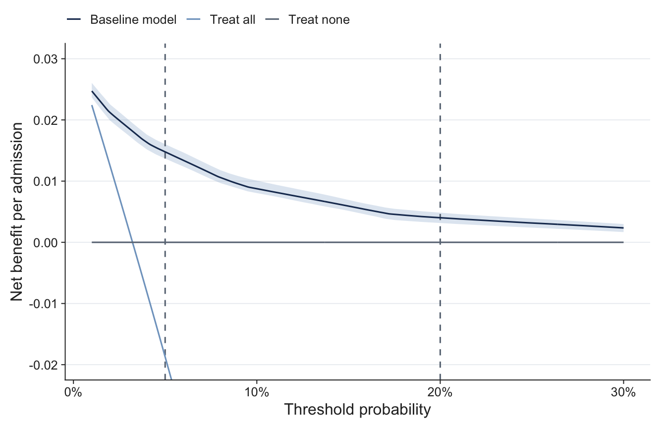
Net benefit at threshold $t$ is the true-positive rate minus the false-positive rate weighted by $t/(1-t)$.
The baseline model has seven binary predictors, so there are only 128 predictor profiles, each with a known
risk. Given the probability of each profile, net benefit at every threshold is an exact calculation: sort
the profiles by risk, flag those at or above $t$, and add up. No patient-level sample is drawn.
The profile probabilities come from numerical integration of the fitted 7-dimensional normal, not from
simulating patients. The integrator (mvtnorm) uses a randomised quasi-Monte Carlo rule internally, with the
error target set to $10^{-7}$ per profile. Repeat runs with different seeds agree to about $10^{-6}$, which
is below any difference that matters here, and the test suite checks this.
The same code takes separate "decision" and "outcome" risks, so once genetic terms enter the data-generating
model it can score a clinical-only rule against the true risk without change.
::: {.callout-important}
## The curve and bands below come from the fitted copula
Since decisions D9 and D10 (18 October 2026), the baseline cohort for the genetic layer is the observed distribution of
the clinical profiles in the 4,078 unique admissions of `boscore.xlsx` (the 49 non-event twin rows removed), with
patients resampled in the bootstrap, and the baseline model is a refit on that cohort. The curve and bands below are
the copula's with the published equation, a sensitivity analysis. The MCID table at the end of this page shows the
adopted refit values next to the earlier ones.
:::
## The baseline decision curve
```{r}
#| label: fig-dca
#| fig-cap: "Net benefit of the fixed baseline model on the fitted cohort. The shaded band is the 90% range across 150 near-optimal correlation matrices. Dashed lines mark the 5% (primary) and 20% (secondary) thresholds."
#| fig-height: 4.5
plot_dca(fit, get_band("nb"), band_fill = jama_cols[["steel"]], mark_col = jama_cols[["grey"]],
         line_cols = c("Baseline model" = jama_cols[["navy"]], "Treat all" = jama_cols[["steel"]], "Treat none" = jama_cols[["grey"]])) +
  theme_jama(base_size = 12)
```
```{r}
#| label: tbl-summary
#| tbl-cap: "Baseline net benefit at the pre-specified thresholds. Ranges are the 5th to 95th percentile across the correlation ensemble."
summ |>
  transmute(
    Threshold = threshold,
    `Net benefit` = nb,
    `Ensemble range` = sprintf("%.4f to %.4f", nb_lo, nb_hi),
    `Treat all` = nb_all,
    `True positives per 1,000` = tp_per_1000,
    `False positives per 1,000` = fp_per_1000,
    Flagged = flagged
  ) |>
  gt() |>
  fmt_percent(c(Threshold, Flagged), decimals = 1) |>
  fmt_number(c(`Net benefit`, `Treat all`), decimals = 4) |>
  fmt_number(c(`True positives per 1,000`, `False positives per 1,000`), decimals = 1)
```
```{r}
#| label: fig-rates
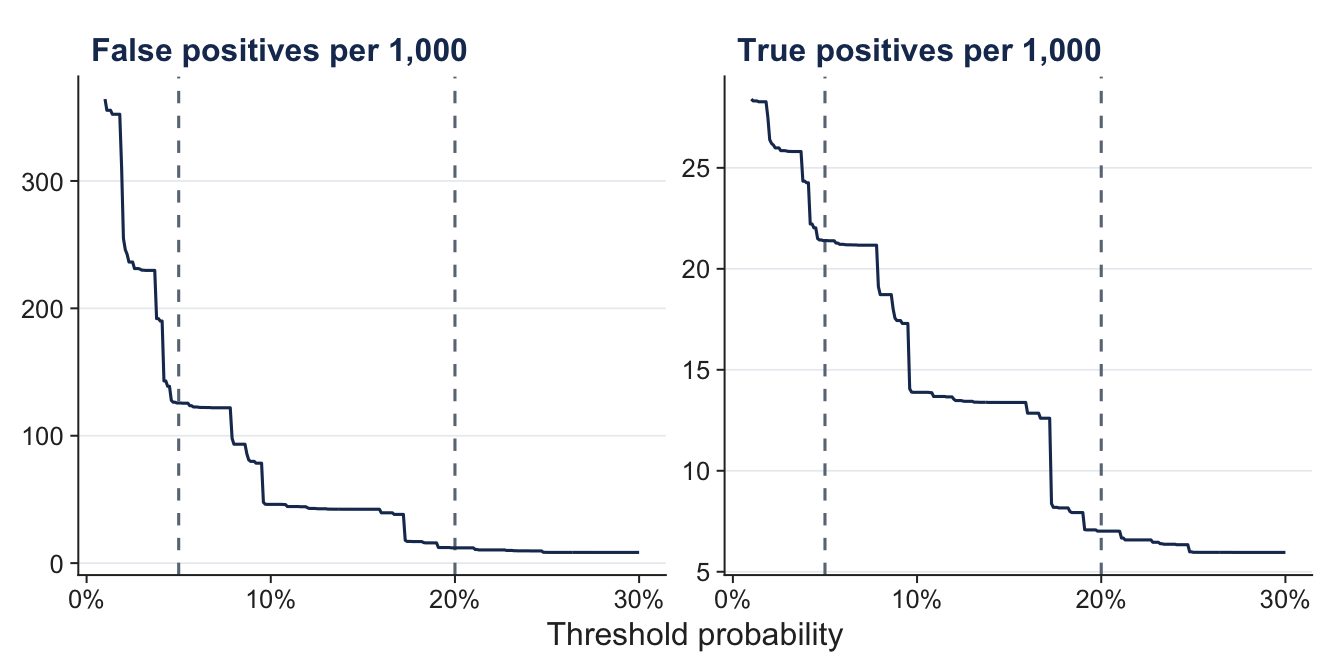
#| fig-cap: "True and false positives per 1,000 admissions as the threshold rises."
#| fig-height: 3.5
plot_dca_rates(fit, line_col = jama_cols[["navy"]], mark_col = jama_cols[["grey"]]) + theme_jama(base_size = 12)
```
The curves are step functions because the 128 profiles carry a limited number of distinct risks. Each
step is a group of profiles dropping below the threshold. Adding genetic terms will split these groups and
smooth the curves.
## The minimum clinically important difference
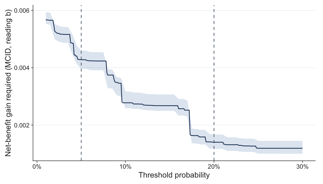
The pre-specified MCID (reading b) is 20% more true cases of invasive mould disease at no increase in false
positives, which in net-benefit terms is 0.2 times the baseline true-positive rate at the threshold. The 5%
threshold is primary, because it is the cut-off the Stanzani paper used to define high risk. The 20%
threshold is secondary.
```{r}
#| label: fig-mcid
#| fig-cap: "Net-benefit gain the genetic layer would have to deliver, by threshold. Shaded band as in the decision-curve figure."
#| fig-height: 4
plot_mcid(fit, get_band("mcid_b"), band_fill = jama_cols[["steel"]], line_col = jama_cols[["navy"]], mark_col = jama_cols[["grey"]]) + theme_jama(base_size = 12)
```
```{r}
#| label: tbl-mcid
#| tbl-cap: "MCID (reading b) on three cohorts."
ref <- read.csv("data/baseline_net_benefit_reference.csv")
q_v1 <- read.csv("output/v1/profile_probabilities.csv")
risk <- plogis(profile_logit(pars, all_profiles()))
v1 <- dca_exact(q_v1$q, risk, thresholds = c(0.05, 0.20))
emp <- read.csv("output/dca_empirical_summary.csv")
base <- read.csv("output/dca_baseline_summary.csv")
refit <- read.csv("output/dca_baseline_refit_summary.csv")
sel <- function(d, col) d[[col]][d$threshold %in% c(0.05, 0.20)]
tibble(
  Threshold = c("5% (primary)", "20% (secondary)"),
  `Indicative (rho = 0.30)` = ref$mcid_b_20pc_more_tp[ref$threshold %in% c(0.05, 0.20)],
  `Copula v1` = v1$mcid_b,
  `Copula v2 (at the lock)` = sel(summ, "mcid_b"),
  `v2 ensemble 5%` = sel(summ, "mcid_lo"),
  `v2 ensemble 95%` = sel(summ, "mcid_hi"),
  `4,127 rows (D8)` = sel(emp, "mcid_b"),
  `Published equation, base cohort (D9)` = sel(base, "mcid_b"),
  `Refit baseline (adopted)` = sel(refit, "mcid_b"),
  `Refit bootstrap 5%` = sel(refit, "mcid_lo"),
  `Refit bootstrap 95%` = sel(refit, "mcid_hi"),
  `Observed outcomes` = sel(base, "observed_mcid")
) |>
  gt() |>
  fmt_number(where(is.numeric), decimals = 5)
```
```{r}
#| label: plateau
i5 <- which(abs(fit$threshold - 0.05) < 1e-9)
ok <- abs(fit$mcid_b / fit$mcid_b[i5] - 1) < 0.05
lo <- i5; while (lo > 1 && ok[lo - 1]) lo <- lo - 1
hi <- i5; while (hi < length(ok) && ok[hi + 1]) hi <- hi + 1
plateau <- fit$threshold[c(lo, hi)]
```
The primary value is stable across the four cohorts (within about 6% of the indicative figure), while the
secondary value falls by about a quarter. The adopted refit-baseline values are +0.00458 at 5% and +0.00160 at 20%. They are higher than the
published-equation values (+0.00404 and +0.00113) because the published equation under-predicts slightly on the
corrected cohort (3.06% predicted against 3.26% observed), so adopting the refit makes the primary test harder for the
genetic layer. Results are also reported against the published-equation and 4,127-row values. The 5% value sits on a plateau: the MCID stays within 5% of its
value at 5% for thresholds from about `r sprintf("%.1f%%", 100 * plateau[1])` to
`r sprintf("%.1f%%", 100 * plateau[2])`. The spread across the ensemble, about plus or minus 7% at 5% and
plus or minus 18% at 20%, is the part that rests on the unpublished correlation structure.
## How much does the MCID depend on the outcome risk?
The published equation was fitted with the 49 twin rows in, and on the corrected cohort it under-predicts slightly
(3.06% predicted against 3.26% observed). So the MCID can be computed under different readings of the "true" outcome
risk. The decision rule is the published equation's, except in scenario C. Patients are resampled, with the refit
repeated inside every resample.
```{r}
#| label: tbl-outcome-risk
#| tbl-cap: "MCID under four readings of the outcome risk, with 90% patient-bootstrap intervals."
sens <- read.csv("output/mcid_outcome_risk_sensitivity.csv")
sens |>
  transmute(Scenario = scenario, Threshold = threshold, MCID = mcid_b, `5%` = mcid_lo, `95%` = mcid_hi,
            `Relative to A` = mcid_relative_to_A, `True positives per 1,000` = tp_per_1000) |>
  gt(groupname_col = "Threshold") |>
  fmt_percent(`Relative to A`, decimals = 0) |>
  fmt_number(c(MCID, `5%`, `95%`), decimals = 5) |>
  fmt_number(`True positives per 1,000`, decimals = 1)
```
The adopted value (A, published equation as truth) is the lowest at every threshold. The alternatives raise the primary
MCID by 9 to 13% and the secondary by 21 to 41%, which makes the adopted reading the most permissive one for the primary
test. The intervals overlap, so the data cannot separate the readings, and the published coefficient lies inside the
refit's interval for every term:
```{r}
#| label: tbl-refit
#| tbl-cap: "Published coefficients against a refit on the 4,078 unique admissions (90% patient-bootstrap interval)."
read.csv("output/refit_coefficients.csv") |>
  transmute(Term = gsub("_", " ", term), Published = published, Refit = refit, `5%` = lo, `95%` = hi) |>
  gt() |>
  fmt_number(2:5, decimals = 2)
```
The 4,127-row MCID (+0.00445 at 5%, +0.00142 at 20%) sits close to the refit-truth and observed-outcome readings, so
reporting against it, as decision D9 commits to, brackets them.
## Using the machinery for the genetic layer
```r
# Cells: clinical profile x genetic class. Decisions use the clinical-only risk;
# outcomes use the true risk including genetics.
base  <- dca_exact(w, risk_true, risk_pred = risk_clinical)
with  <- dca_exact(w, risk_true, risk_pred = risk_with_genetics)
dca_compare(base, with)   # delta_nb, the baseline MCID, and whether it is met
```
`dca_compare()` takes the MCID from the baseline curve, so the test is fixed by the baseline and cannot
drift with the candidate model.
## Limitations
- Results are for the baseline alone. No genetic term has been added.
- The ensemble spread reflects only the correlation structure. It does not include uncertainty from
admission clustering or from using the apparent aROC of 0.85.
- Net benefit is per admission. Patients with several admissions contribute correlated events, which
matters for uncertainty but not for the exact point values here.