---
title: "Evidence mapping"
subtitle: "From extracted studies to model parameters: PTX3, CLEC7A, TLR4, CD209, IL10 and IFNG"
date: today
---
```{r}
#| label: setup
source("_setup.R")
studies <- read.csv("output/ptx3_study_effects.csv")
pooled  <- read.csv("output/ptx3_h2_pooled.csv")
cross   <- read.csv("output/ptx3_snp_crosscheck.csv")
donor   <- read.csv("output/ptx3_donor_effects.csv")
rows    <- read.csv("output/ptx3_row_effects.csv")
vlog    <- read.csv("output/ptx3_verification_log.csv")
s035    <- read.csv("output/s035_direction_check.csv")
s029    <- read.csv("output/s029_genotype_frequency_check.csv")
clec    <- list(study = read.csv("output/clec7a_study_effects.csv"), pooled = read.csv("output/clec7a_pooled.csv"), rows = read.csv("output/clec7a_row_effects.csv"))
tlr4    <- list(study = read.csv("output/tlr4_study_effects.csv"), pooled = read.csv("output/tlr4_pooled.csv"), cross = read.csv("output/tlr4_snp_crosscheck.csv"))
cd209   <- list(study = read.csv("output/cd209_study_effects.csv"), pooled = read.csv("output/cd209_pooled.csv"), cross = read.csv("output/cd209_snp_crosscheck.csv"), rows = read.csv("output/cd209_row_effects.csv"))
il10    <- list(study = read.csv("output/il10_study_effects.csv"), pooled = read.csv("output/il10_pooled.csv"))
ifng    <- list(study = read.csv("output/ifng_study_effects.csv"), pooled = read.csv("output/ifng_pooled.csv"))
strand  <- read.csv("data/rs7309123_strand_resolution.csv")
clec2   <- read.csv("output/clec7a_second_pooled.csv")
study_label <- function(d) paste0(sub(",.*", "", d$first_author), " ", d$year)
```
::: {.callout-warning}
## Provisional
The extraction rows are round 1 plus the recorded corrections. Two papers (Herrero-Sanchez 2018 and Brunel 2018) were read against the
extraction by the assistant. The human round-2 check is reported to have confirmed the extraction against the source PDFs, but its record
is not in the repository. Most mapping rules and the priors are proposals, set out in addenda 7 to 9 of the decision record. Treat every
number on this page as provisional.
:::
## What "h2" means
PTX3 has three loci in strong linkage (rs2305619, rs3816527, rs1840680). In the phased 1000 Genomes European data the common
haplotypes are G-A-G (54%), A-C-A (40%) and A-A-A (6%), with alleles in that locus order.
- **h2 is the chromosome class that carries the A allele at rs2305619**: A-C-A, A-A-A and the very rare A-A-G, 45.6% in
1000G EUR and 48.2% in gnomAD NFE. **h1 is G-A-G.** The model term is an additive per-copy effect of h2 in the recipient.
- **rs1840680 A is the same class** (r² = 0.996), so it is an interchangeable tag.
- **rs3816527 C is not interchangeable.** It marks only A-C-A, about 87% of h2, so evidence reported on it is mapped to h2
through the haplotype structure and used as a cross-check.
## How each study is converted
Studies report PTX3 in different ways: dominant or recessive contrasts, allelic odds ratios, or genotype counts, with the
contrast sometimes written in both directions. Each one is converted to a single scale, the log odds ratio per h2 copy, by
finding the effect that a haplotype model would need to produce the study's contrast. The model is additive on the log-odds
scale, uses Hardy-Weinberg haplotype pairs and case-control sampling, and the standard error follows by the delta method.
The direction of each contrast is read from the comparison text, including which side is the reference.
## One effect per study
```{r}
#| label: tbl-studies
#| tbl-cap: "Primary analysis: recipient genotype, odds-ratio scale, whole-cohort analyses, without Herrero-Sanchez 2018."
studies |>
  transmute(Study = paste0(sub(",.*", "", first_author), " ", year), `Evidence used` = paste(tier, model, sep = ", "),
            `Log OR as reported` = y, `Per-copy h2 effect` = beta, SE = se_beta, `OR per h2 copy` = or_per_h2_copy,
            Note = flag) |>
  gt() |>
  fmt_number(c(`Log OR as reported`, `Per-copy h2 effect`, SE, `OR per h2 copy`), decimals = 2)
```
```{r}
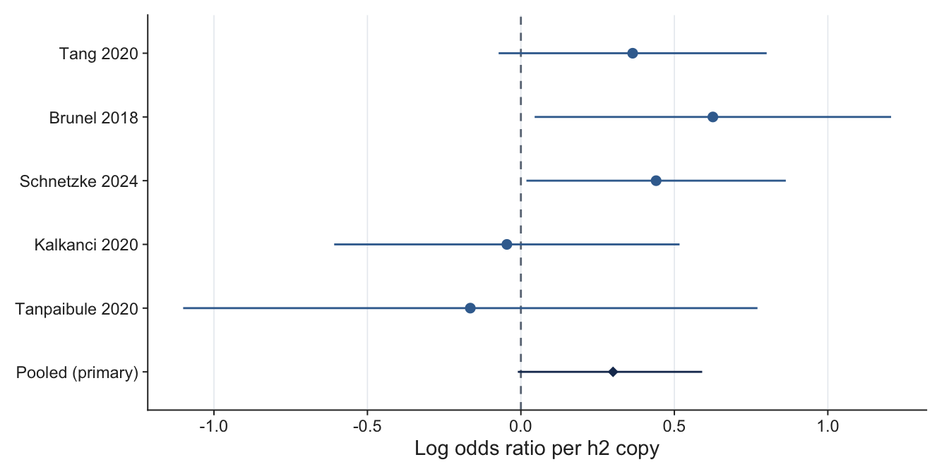
#| label: fig-forest
#| fig-cap: "Per-copy h2 effect for each study (90% interval) and the pooled estimate with its 90% credible interval."
#| fig-height: 3.5
pr <- pooled[1, ]
d <- bind_rows(
  studies |> transmute(label = paste0(sub(",.*", "", first_author), " ", year), est = beta, lo = beta - 1.645 * se_beta, hi = beta + 1.645 * se_beta, kind = "Study"),
  tibble(label = "Pooled (primary)", est = pr$mu, lo = pr$mu_lo, hi = pr$mu_hi, kind = "Pooled")
)
d$label <- factor(d$label, levels = rev(d$label))
ggplot(d, aes(est, label, shape = kind)) +
  geom_vline(xintercept = 0, linetype = "dashed", colour = jama_cols[["grey"]]) +
  geom_pointrange(aes(xmin = lo, xmax = hi, colour = kind)) +
  scale_shape_manual(values = c(Study = 16, Pooled = 18)) +
  scale_colour_manual(values = c(Study = jama_cols[["blue"]], Pooled = jama_cols[["navy"]])) +
  labs(x = "Log odds ratio per h2 copy", y = NULL, shape = NULL) +
  theme_jama(grid = "x") + theme(legend.position = "none")
```
## Pooled effect
```{r}
#| label: tbl-pooled
#| tbl-cap: "Bayesian random-effects pooling, with sensitivity analyses. mu ~ N(0, 1) and tau ~ half-normal(0.5) on the log-odds scale."
pooled |>
  transmute(Analysis = scenario, Studies = k, `Log OR` = mu, `5%` = mu_lo, `95%` = mu_hi, OR = or, `OR 5%` = or_lo, `OR 95%` = or_hi,
            tau = tau, `P(effect < 0)` = prob_below_zero) |>
  gt() |>
  fmt_number(c(`Log OR`, `5%`, `95%`, OR, `OR 5%`, `OR 95%`, tau), decimals = 2) |>
  fmt_percent(`P(effect < 0)`, decimals = 0)
```
The primary estimate is an odds ratio of `r sprintf("%.2f", pooled$or[1])` per h2 copy, with a 90% interval of
`r sprintf("%.2f", pooled$or_lo[1])` to `r sprintf("%.2f", pooled$or_hi[1])`. The interval just reaches 1, and the prediction
interval for a new study is wide (an odds ratio of `r sprintf("%.2f", exp(pooled$pred_lo[1]))` to `r sprintf("%.2f", exp(pooled$pred_hi[1]))`),
so the evidence is weak. Herrero-Sanchez 2018 first appeared to point the other way; reading the paper showed that the extraction followed a
reference label that is reversed in the source, and corrected it is positive (see the next section). Adding it
raises the estimate and tightens the interval, and dropping Brunel 2018 lowers the estimate and widens it.
## Checking rows against their sources
Two studies drive most of the doubt about direction, so they were read first.
```{r}
#| label: tbl-verification
#| tbl-cap: "What was checked, what the source says, and what follows. Herrero-Sanchez 2018 was read as full text; Brunel 2018 from a summary of the article page, so its figures are not verbatim."
vlog |>
  transmute(Study = study, Item = item, `The source says` = source_says, Verdict = verdict, Consequence = consequence) |>
  gt() |>
  tab_options(table.font.size = "small")
```
**Herrero-Sanchez 2018.** In every table the reference group is labelled 1.00, but the printed odds ratio belongs to that group
against the others. The genotype counts show it for every SNP and model checked:
```{r}
#| label: tbl-s035
#| tbl-cap: "Herrero-Sanchez 2018: the printed odds ratio against the crude odds ratio from the genotype counts, in each direction. Reading A: the reference-labelled group is the numerator. Reading B: the other group is."
s035 |>
  transmute(Table = table, SNP = snp, Model = model, Printed = printed_or, `Crude, reading A` = crude_ref_vs_other,
            `Distance, A` = distance_if_reference_numerator, `Distance, B` = distance_if_other_numerator,
            Decisive = ifelse(decisive, "yes", "no")) |>
  gt() |>
  fmt_number(c(Printed, `Crude, reading A`, `Distance, A`, `Distance, B`), decimals = 2)
```
All 18 comparisons favour reading A (16 decisively, 2 too close to 1 to tell). The extracted study therefore has a positive per-copy
h2 effect, like the others.
**Brunel 2018.** The extracted counts for the group labelled "homozygous for the minor allele" can be compared with what
Hardy-Weinberg predicts from the paper's own minor allele frequencies (0.48 for rs2305619, 0.44 for rs3816527):
```{r}
#| label: tbl-s029
#| tbl-cap: "Brunel 2018: the share of courses in the extracted homozygote group, against the minor-allele and major-allele homozygote shares that Hardy-Weinberg predicts."
s029 |>
  transmute(SNP = rsid, Analysis = analysis, Observed = observed, `Expected, minor homozygotes` = expected_minor_homozygotes,
            `Expected, major homozygotes` = expected_major_homozygotes, `z, minor` = z_minor_homozygotes, `z, major` = z_major_homozygotes) |>
  gt() |>
  fmt_number(2:7, decimals = 2)
```
For rs3816527 the extracted group fits the major-allele homozygotes and not the minor ones (z about 3 to 4), in every stratum. So the
group may not be the one the paper describes, and the sign of this study's effect is not secure. The per-SNP counts themselves are
only in a supplementary figure.
```{r}
#| label: tbl-unmapped
#| tbl-cap: "Why usable PTX3 rows do not map to a per-copy h2 effect."
tab <- table(Reason = ifelse(is.na(rows$beta), sub(";.*", "", rows$flag), "mapped"))
tibble(Reason = names(tab), Rows = as.integer(tab)) |> arrange(desc(Rows)) |> gt()
```
## Does the h2 definition hold?
If h2 explains the signal, mapping a study through rs3816527 instead of the h2 tag SNP should give about the same per-copy
effect.
```{r}
#| label: tbl-cross
#| tbl-cap: "The same study mapped through the h2 tag SNP and through rs3816527."
cross |>
  transmute(Study = study_id, `Through the h2 tag SNP` = beta_tag, `Through rs3816527` = beta_rs3816527, Difference = difference) |>
  gt() |>
  fmt_number(2:4, decimals = 2)
```
The two agree to within about 0.15 for every study, which supports defining h2 by the rs2305619 and rs1840680 A alleles.
## Donor genotype
Donor genotype is the pre-specified secondary analysis (allogeneic HSCT only). Only one study reports it, so it is described
and not pooled.
```{r}
#| label: tbl-donor
#| tbl-cap: "Donor-genotype evidence, mapped to a per-copy h2 effect."
donor |>
  transmute(Study = paste0(sub(",.*", "", first_author), " ", year), Evidence = paste(tier, model, measure, sep = ", "),
            `Per-copy h2 effect` = beta, SE = se_beta, `OR per h2 copy` = or_per_h2_copy) |>
  gt() |>
  fmt_number(3:5, decimals = 2)
```
## CLEC7A: the Y238X haplotype
Y238X (the C allele of rs16910526 on the forward strand) sits only on the C-G haplotype of rs16910526 and rs7309123, which is
7.7% of chromosomes in gnomAD NFE (A-G is 34.9% and A-C 57.4%). The term is the per-copy effect of that haplotype. Studies that
write the allele as G are on the opposite strand, and are complemented.
```{r}
#| label: tbl-clec7a
#| tbl-cap: "CLEC7A, primary analysis: one effect per study, per copy of the Y238X haplotype."
clec$study |>
  transmute(Study = paste0(sub(",.*", "", first_author), " ", year), `Evidence used` = paste(tier, model, sep = ", "),
            `Log OR as reported` = y, `Per-copy effect` = beta, SE = se_beta, `OR per copy` = or_per_copy) |>
  gt() |>
  fmt_number(c(`Log OR as reported`, `Per-copy effect`, SE, `OR per copy`), decimals = 2)
```
```{r}
#| label: tbl-clec7a-pooled
#| tbl-cap: "CLEC7A pooled effect."
clec$pooled |>
  transmute(Analysis = scenario, Studies = k, OR = or, `OR 5%` = or_lo, `OR 95%` = or_hi, tau = tau) |>
  gt() |>
  fmt_number(c(OR, `OR 5%`, `OR 95%`, tau), decimals = 2)
```
Among the small odds-ratio studies Y238X is null. The largest study (Fisher 2017, 483 cases) reports hazard ratios above 1, and
including it moves the pooled effect up. **The second CLEC7A effect** is the per-copy effect of the A-G haplotype, the G allele of rs7309123 on the non-Y238X background (A-C is the reference). rs7309123 is a C/G
palindrome, so the strand each study used had to be determined from its control frequencies and the papers themselves; the evidence for each study is in
`data/rs7309123_strand_resolution.csv` and in addendum 16 of the decision record. Studies are graded A to D, and only grades A and B (resolved with at least low-to-medium confidence; the full texts of Kalkanci 2020 and Chen 2019 settled their strands, addendum 19)
enter the primary estimate.
```{r}
#| label: tbl-strand
#| tbl-cap: "Strand of rs7309123 in each study that reports it. The likelihood ratio compares the study's control frequency of the labelled allele with the forward-strand and opposite-strand reference frequencies."
strand |>
  transmute(Study = paste0(first_author, " ", year), Ancestry = ancestry, `Labelled allele frequency` = observed_frequency_of_labelled_allele,
            `log10 LR, forward vs opposite` = log10_likelihood_ratio_forward_vs_opposite, Conclusion = strand_conclusion, Grade = grade) |>
  gt() |>
  fmt_number(c(`Labelled allele frequency`, `log10 LR, forward vs opposite`), decimals = 2) |>
  sub_missing(missing_text = "")
```
```{r}
#| label: tbl-clec2
#| tbl-cap: "The second CLEC7A parameter (OR per A-G copy), with Y238X held at its pooled effect. Non-European studies are left out of the primary analysis because the European haplotype frequencies do not describe them."
clec2 |>
  transmute(Analysis = scenario, Studies = k, OR = or, `OR 5%` = or_lo, `OR 95%` = or_hi, tau = tau) |>
  gt() |>
  fmt_number(c(OR, `OR 5%`, `OR 95%`, tau), decimals = 2)
```
The primary estimate rests on three studies (Schnetzke 2024, Kalkanci 2020 and Sainz 2012) and is an odds ratio of `r sprintf("%.2f", clec2$or[1])` per A-G copy, with a 90% interval from `r sprintf("%.2f", clec2$or_lo[1])`
to `r sprintf("%.2f", clec2$or_hi[1])`. The interval excludes 1 in every analysis. Adding the Jena cohort, whose strand is only weakly resolved, gives `r sprintf("%.2f", clec2$or[clec2$scenario == "adding the Jena cohort (grade C)"])`, and taking every study as forward strand gives `r sprintf("%.2f", clec2$or[clec2$scenario == "all studies, unresolved ones taken as forward"])`. The row that adds the non-European studies is not a valid estimate (their contrasts are mapped through European haplotype frequencies) and is shown only to document why they are excluded.
## TLR4: the G-T haplotype
The term is the G-T haplotype of rs4986790 (G) and rs4986791 (T), 6.1% of chromosomes in gnomAD NFE. No cohort has minor
homozygotes, so every study enters as carriers against non-carriers, with 0.5 added to a zero cell (decision D3c).
```{r}
#| label: tbl-tlr4
#| tbl-cap: "TLR4, primary analysis: one effect per study, per copy of the G-T haplotype."
tlr4$study |>
  transmute(Study = paste0(sub(",.*", "", first_author), " ", year), SNP = rsid, `Log OR as reported` = y, `Per-copy effect` = beta,
            SE = se_beta, `OR per copy` = or_per_copy) |>
  gt() |>
  fmt_number(c(`Log OR as reported`, `Per-copy effect`, SE, `OR per copy`), decimals = 2)
```
```{r}
#| label: tbl-tlr4-pooled
#| tbl-cap: "TLR4 pooled effect."
tlr4$pooled |>
  transmute(Analysis = scenario, Studies = k, OR = or, `OR 5%` = or_lo, `OR 95%` = or_hi, tau = tau) |>
  gt() |>
  fmt_number(c(OR, `OR 5%`, `OR 95%`, tau), decimals = 2)
```
The effect is positive but uncertain. The two SNPs disagree within a large sampling error, which is expected from carrier counts this
small. de Boer 2011 analysed donors and recipients and the extraction does not say which genotype its rows use, so it is left out
of the primary analysis; treating it as a recipient study raises the estimate. Tanpaibule's allele is carried by none of its 33 cases
against 11 of 295 controls, so its estimate rests on the continuity correction.
## CD209: G at rs4804800
The two CD209 SNPs (rs4804800 and rs7248637, r² = 0.41) give four haplotypes in gnomAD NFE: G-A 7.8%, A-A 2.6%, G-G 4.7% and A-G 84.9%.
The term is the per-copy effect of the chromosome class that carries G at rs4804800 (G-A and G-G, 12.5%). rs4804800 rows map to it
directly. rs7248637 rows (the A allele) map through the haplotype structure and are used where a study has no rs4804800 row.
A second CD209 parameter is not estimated.
```{r}
#| label: tbl-cd209
#| tbl-cap: "CD209, primary analysis: one effect per study, per copy of the rs4804800 G class. Hazard-ratio studies are a sensitivity analysis because three odds-ratio studies meet the threshold."
cd209$study |>
  transmute(Study = study_label(cd209$study), SNP = rsid, `Evidence used` = paste(tier, model, sep = ", "), `Log OR as reported` = y,
            `Per-copy effect` = beta, SE = se_beta, `OR per copy` = or_per_copy) |>
  gt() |>
  fmt_number(c(`Log OR as reported`, `Per-copy effect`, SE, `OR per copy`), decimals = 2)
```
```{r}
#| label: tbl-cd209-pooled
#| tbl-cap: "CD209 pooled effect."
cd209$pooled |>
  transmute(Analysis = scenario, Studies = k, OR = or, `OR 5%` = or_lo, `OR 95%` = or_hi, tau = tau) |>
  gt() |>
  fmt_number(c(OR, `OR 5%`, `OR 95%`, tau), decimals = 2)
```
The effect is positive in all three studies. The two studies that also report rs7248637 agree with their rs4804800 effect
(differences of `r paste(sprintf("%.2f", cd209$cross$difference), collapse = " and ")` on the log scale), which supports mapping the
rs7248637 evidence to the same class. Adding Fisher 2017 (hazard ratios, rs7248637) lowers the pooled odds ratio to
`r sprintf("%.2f", cd209$pooled$or[cd209$pooled$scenario == "with hazard-ratio studies"])`, with an interval that includes 1.
Sainz 2011's two rows cannot be mapped: an allele is missing and the comparison has more than two groups.
## IL10 and IFNG: dropped from the panel
IL10 rs1800896 and IFNG rs2069705 are single SNPs. The risk allele is the forward-strand allele that most studies report as their effect
allele (IL10 C, reported as G; IFNG G, reported as C), and a study that reports the other allele is mapped to the same class with the sign
reversed. Both were mapped as optional terms, then **dropped from the panel on 19 October 2026 (addendum 10)** because the evidence is too thin
to estimate an effect.
```{r}
#| label: tbl-optional
#| tbl-cap: "IL10 and IFNG: odds-ratio evidence has fewer than three studies, so hazard-ratio studies were added (the fallback rule); the pooled value is mostly the prior."
bind_rows(
  il10$study |> mutate(Term = "IL10 rs1800896 C", Study = study_label(il10$study)),
  ifng$study |> mutate(Term = "IFNG rs2069705 G", Study = study_label(ifng$study))
) |>
  transmute(Term, Study, `Evidence used` = paste(tier, model, measure, sep = ", "), `Per-copy effect` = beta, SE = se_beta, `OR per copy` = or_per_copy) |>
  gt() |>
  fmt_number(c(`Per-copy effect`, SE, `OR per copy`), decimals = 2)
```
```{r}
#| label: tbl-optional-pooled
#| tbl-cap: "IL10 and IFNG pooled effect, first row of each term is the primary (fallback) analysis."
bind_rows(il10$pooled |> mutate(Term = "IL10"), ifng$pooled |> mutate(Term = "IFNG")) |>
  transmute(Term, Analysis = scenario, Studies = k, OR = or, `OR 5%` = or_lo, `OR 95%` = or_hi, tau = tau) |>
  gt() |>
  fmt_number(c(OR, `OR 5%`, `OR 95%`, tau), decimals = 2)
```
IL10 rests on one study (Tanpaibule 2020, a dominant odds ratio of about 5), so its pooled value is that study shrunk by the prior; adding
de Boer 2011, whose genotype source is unstated, gives two studies. The two IFNG studies disagree in direction, and the hazard-ratio
fallback adds nothing because Fisher's IFNG rows are donor genotype only. Putting either term back would be a sensitivity analysis.
## Limits
- The rows are unverified except where stated above, and the checks so far are the assistant's, not the human round-2 check.
- Brunel 2018 states "the minor allele", so its effect allele is inferred from European frequencies, and the frequency check above
casts doubt on it.
- The Chinese and Thai cohorts use European haplotype frequencies.
- Three to five studies per term is few. The priors on the pooled effect and on tau are proposals.
- Open questions from addendum 8 that the human checks did not settle: whether to use Herrero-Sanchez's invasive aspergillosis rows
and whether to keep Brunel in the primary analysis. The rs7309123 strand is resolved with some confidence for six of the ten studies and weakly for three more; only Zhao 2022 is undetermined (addenda 16 and 19). Hazard-ratio studies join a term's primary
analysis only when it has fewer than three odds-ratio studies (addendum 9).